Guzman Y Gomez Business Intelligence

I had the pleasure of working with my favourite Mexican restaurant chain, Guzman Y Gomez. Their tacos are amazing. I like to think that I helped them in a small way by allowing them to report and analyse combined data close to real time.

Guzman Y Gomez - business intelligence case study.

Memory is Oxygen for Large Database Systems

I am frequently invited in to assist with database (OLTP, DW and OLAP) performance, and often the issue is IO throughput related. So, the solution tends to involve tuning queries (and indexes) to reduce IO or improving the IO capacity of the SAN (or both). Of course, in all of these IO related performance issues, RAM can be a great elixir. Databases love memory. They are designed to use RAM by holding popular pages, compiled plans and work tables in memory. So, if you have a large database with a performance issue; very quick, and relatively cheap relief might be gained simply by adding RAM.

SQL Server is particularly good at exploiting available RAM - and (just as important) reducing memory demands if the operating system is paging. With the default SQL install options, all you need to do is give RAM to the OS and SQL will use it to hold more data and plans in memory. Sometimes this can be an exponential beneficial effect since, by reducing IO demands, the SAN is no longer a bottleneck and remaining IO is executed much faster.

Multidimensional OLAP databases also like to have lots of RAM. Even larger than the combined OLAP database size! See earlier blog. Unfortunately, SQL Server OLAP is not as memory effective as the relational SQL, but it will hold data (and aggregations) in memory, improving query and processing performance. SQL Tabular is an exception, as it requires the entire cube to reside in memory. It will simply not work without sufficient memory.

RAM, by and large, has no licencing cost with SQL Server, which can be a big consideration. Adding CPUs will generally incur significant OS and SQL licensing costs. I said, by and large, since with SQL 2012 and SQL 2014, there are, unfortunately, limits on SQL Server Standard Edition memory.

• SQL 2008 Standard Edition has no memory limit
• SQL 2012 Standard Edition has 64GB memory limit
• SQL 2014 Standard Edition has 128GB memory limit
• (SQL Server Enterprise Edition versions support their OS limits)

So, if you have a performance issue with a large database, and can't wait for a database tuning expert; before adding CPUs, Fusion IO cards etc.; try giving your system more RAM.

Database IO Throughput

I've written on this before, but I feel I need to say it again in a different way as so many people fail to grasp the significance of IO throughput capacity.  If you see messages in the SQL log along the lines of the following, then you have a very very serious IO throughput issue. I didn't make these logs up.  They are real logs!

The best analogy I can draw is if you can imagine your company has 1000 staff and you have a building of 20 floors with 4 lifts that can adequately house all staff.  Your 1000 staff tend to drift in between 9 and 10AM and the 4 lifts can move the 1000 staff to their desired floors in the hour.  Infrequently, staff will queue for a lift as the first lift will be full, but it's rarely longer than one lift ride for the wait.  During the day, the lift demands are lower and there are no queues.

Now, over time, your company grows to 2500 staff, and you've added another 30 floors to your building and the lifts are extended to cater for all 50 floors.  The CEO is relieved that the building capacity has been increased to house the new staff and that the lifts work across all 50 floors.  However, no one has thought about the increased throughput required by the lifts.  Between 9 and 10AM 2500 staff now drift into the office and want a lift to their floors, however the 4 lifts are only capable of moving about 1200 staff/hour.  The queues for the lifts build up and are not fully drained until after 11AM.  The company is now in trouble with disgruntled staff and find it needs to ask staff to come in earlier or later.  Also, there is the hidden issue of the fire exit stairways also having throughput limits.  With 1000 staff, the building could be evacuated in 15 minutes, now with 2500 staff (and the same stairways) it will take over 40 minutes.

This is analogous to a SQL Server database growing over time, and the SAN (playing the role of the lifts) is extended to hold more TeraBytes, but its throughput capacity (measured in MegaBytes/second of reading and writing) is not increased.  The IO queues start to build up and IO times degrade.  The SQL Log picture above is an example where hundreds of IO every minute are taking longer than 15 seconds to complete!  This is an unbelievably dire situation that can cause SQL Server to shutdown. 

I am not advising that you monitor your SQL Server log for long running IOs, although if you see them, you should act immediately.  I advise you to monitor IO throughput, average latency, and queue length continually, using Perfmon or related tool.  You can detect throughput capacity when MB/second tends to flatline while IO latency and queue lengths are waxing and waning.  Unfortunately, Perfmon, is not a complete tool, but it does have all the base information and there are many third party tools, or you can do what I do and create your own by having Perfmon send records to a common SQL Server database and cube.  You only need a few counters and only record every 60 seconds, or so.  If the Perfmon database is on another server, there will be very little load on your production servers, essentially no IO.  Your Perfmon database could hold performance data for all your production servers, so that you have all the performance information you need in one place.  Also, when you have a performance issue you have historical information of this issue and trends earlier in time.  Companies that don't continually record these metrics are flying somewhat blind, or, at least, flying with blinkers on.  Here's an earlier blog on creating a Perfmon cube, although, unfortunately, the online demonstration is no longer available.  

This posting is not intended to provide answers to the IO throughput issue.  The solution can be many and varied.  The solution will probably involve speeding up the storage system, but it might be to make the database more IO efficient.  The most important point I can make is that you should be monitoring and be able to recognise this issue.  Also, don't let a storage person tell you that you have hit the maximum possible throughput.  There are always ways to increase the throughput performance of your storage, as there are always ways to improve your database performance.

Cube processing goes slow when there are dimension key errors

I try and keep my cubes as clean as possible, so that dimension key errors are minimised. However, as a safeguard I tend to enable UnknownMembers. This way the totals are correct even if the customer, item, cashier etc isn't found in the dimension. 

Unfortunately, SSAS (2008 R2) still consumes quite a lot of cpu dealing with these UnknownMembers. This is fine if you only have a few million facts to process, but if you have billions (or even just hundreds of millions) processing noticeably slows down. This manifests as a single cpu busy in msmdsrv. The difference in cube processing time can be by a factor of 20, or so. My rule of thumb is that a partition should be able to process tens of millions of facts per minute. However, if there are key errors, this might drop to less than a million per minute.

If you have configured the ErrorConfiguration to "IgnoreError" you won't even see any error messages when you process in the foreground. But the cpu overhead is still there. The same goes for KeyErrorLimit, cpu will continue to be consumed even though it has stopped logging.

My suggestion is to try, as much as possible, to avoid dimension key errors. A simple coalesce(DimKey,-1) with a "unknown" key value (-1) as the last parameter value, combined with a "unknown" (-1) dimension member. Of course, you don't have to remove every dimension key error, just ensure that there aren't millions (or billions) of them.

My SSAS databases are corrupted

Did you happen to have a unplanned shutdown?  This is quite likely to be the cause of the failure.  This is unlike SQL Server, which has a transaction log and will always recover databases on restart.
As I have mentioned earlier, SQL Server Analysis Services exploits the Windows File Cache to help minimise IO, which might lead you to suspect the Windows cache.  However SSAS uses the FlushFileBuffers API to minimise the possibility of having dirty pages in the Windows File Cache.  However, this does not protect SSAS from corruption on an unplanned shutdown.
So, if you really want to avoid corrupted SSAS databases on power failure, you should ensure your SSAS servers are supported by UPS.
Most production SSAS servers have UPS.  But, if you don't have UPS, like my demonstration site (http://RichardLees.com.au/Sites/Demonstrations) and, like my site, the cubes are continually updating, when the power fails, SSAS databases have a good chance of being corrupted.  The only solution to this, that I know of, is to restore the affected (typically all) SSAS databases.  I find the quickest way to do this is to stop SSAS, empty the SSAS data directory, start SSAS and recover all the databases.  One thing you will also need to do is add back any userids that had SSAS administrator privileges as they were held in a file on the SSAS data directory.

Why doesn't SSAS cache the entire cube?

Would you expect a 36GB server dedicated to SSAS to eventually cache an entire 11GB cube in memory?  If so, you would be wrong.  SSAS does not necessarily keep aggregations in memory, even though memory used is less than Memory\LowMemoryLimit.

I have seen this effect on many production servers but never quite believed it.  There is much more RAM than cube size, yet SSAS is continually losing data from cache and asking for physical IO.  Actually, SSAS relies on the Windows File Cache to reduce much of its IO.  However, the Windows File Cache does not cache the entire cube either.

To demonstrate this effect, I have set up a 36GB server, dedicated to SSAS, and set up an 11GB MOLAP cube.  Then, over a period of 19 hours, I have client tasks querying the cube in a semi random fashion.  The MOLAP cube was not updated over the period.  Over the 19 hours, if SSAS or Windows File Cache were effective, there wouldn't be much more than 11GB of read IO on the SSAS data drive over the 19 hours.  However, the system reached an equilibrium, where it was requesting over 20MB of read IO/second.  If you add this up, the system read 1.3 terabytes of data from the 11GB cube (20MB*60*60*19).  Obviously, the system was not effectively caching the cube.  This is very different from SQL Server, which would quite happily keep an 11GB database in memory, effectively eliminating further read IO.

My server was running Windows 2008, SQL Server 2008 R2 with default configuration settings.  The SSAS database was located on the d: drive.  Nothing else is located on the d: drive
Here is a Perfmon chart with some of the key counters during my test.
SSAS (msmdsrv.exe) did not use more than 12GB of memory during the test, which is well below the LowMemoryLimit 65% (which is about 23GB).

During the 19 hours, SSAS requested, on average, 102MB/second of read IO.  The Windows File Cache was able to satisfy about 80% of these read requests, so the physical disk bytes/second was only 20MB/second. 

The Perfmon chart above shows some of the key counters.  Notice

• The Process (msmdsrv) Bytes/second y axis scale is in MB, often going off scale at 100MB/sec. These are not necessarily physical IO, as the Windows cache will satisfy many.
• The PhysicalDisk Bytes/second is averaging 20.1MB/second for the 19 hours
• The Windows Cache Bytes is sitting between 0.6GB and 1.1 GB.
• The red line (Cache Copy Reads/sec) is the IO requested of the cache.  These are IO that the Windows cache has managed to satisfy by finding the page in its cache.
• See how the Cache Copy Reads/sec is satisfying IO requested of the msmdsrv process, reducing the PhysicalDisk Bytes/sec.  Not so easy to see, as the reads are reads/sec, while the PhysicalDisk and Process are in bytes/sec, but you can see it.

Now that I understand this effect, I am much more appreciative of the Windows Cache.  This is very different from a SQL Server system, where the Windows Cache has little to do as SQL disables the Windows File Cache for its database files.

However, you can clearly see that SSAS (or the system) is performing much more IO than would be necessary if the entire 11GB cube was cached in memory.
There are a couple of takeaways from this exercise

1. Be thankful that we have a Windows Cache, and consider configuring it for SSAS.
2. Try and put SSAS databases on very fast (ideally solid state disks) storage devices.  If you can't avoid the IO, at least make it fast.
3. Partition large cubes.  This helps reduce logical IO requests and to the extent it bunches the popular data together it will probably help the Windows Cache hold the hot data more effectively.
4. Hopefully, in a future version, either SSAS or the Windows File Cache will cache more of the cube.

By the way, this effect is not always noticeable.  If your cube is less than 2-3GB, then it is likely to be well cached between SSAS and Windows File Cache.  Also, if you cube is much larger than the memory available to SSAS, then you would expect to see continual IO, and it is likely to be quite well optimised.  However, when you have a 64 bit server with a cube that is larger than 3GB but is comfortably less than the server memory, you might be surprised to see the volume of continual IO.

Please help get this fixed by voting on https://connect.microsoft.com/SQLServer/feedback/details/760107/multidimensional-cube-is-not-retained-in-memory-even-though-there-is-plenty-of-ram

Improving MDX join performance

Analysis Services will tend to instantiate sets created from joins. Some sets can be extremely large and will actually fail with insufficient resources.
Server: The operation has been cancelled.


The solution is to write the MDX query in such a way that the intermediate sets are smaller. Here is an example of a problematic query that is asking for the top 10 hour/City/Date combinations. The output is simply 10 rows, but AS must create a set with hundreds of Millions of members to get the top 10.

select
[Measures].[Bytes Total] on Columns,
topcount(
[Client Host].[Client Geography].[City]
*[HoursOfDay].[HoursOfDay].[Hour Of Day]
*[Date].[Year Month Day].[Day]
,10,[Measures].[Bytes Total])
on Rows
from EasternMining

Here is a way to improve performance using the generate() function, another one of my favourite MDX functions.

select
[Measures].[Bytes Total] on Columns,
topcount(
generate([Client Host].[Client Geography].[City]
,{[Client Host].[Client Geography].currentmember}
*[HoursOfDay].[HoursOfDay].[Hour Of Day]
*[Date].[Year Month Day].[Day])
,10,[Measures].[Bytes Total])
on Rows
from EasternMining

The generate statement is breaking the query into a couple of steps, so that the largest set will probably be the Days*Hours, from which it is only keeping the top 10 for each city. The outside set, for every city, will only have 10 rows per city. The query is logically equivalent to the first query, meaning it will return the same results.

We could take this logic further with a second generate statement so the inside query only has 1o rows per city day combination.

select
[Measures].[Bytes Total] on Columns,
topcount(
generate([Client Host].[Client Geography].[City]
,topcount(
generate([HoursOfDay].[HoursOfDay].[Hour Of Day]
,topcount({[HoursOfDay].[HoursOfDay].currentmember}
*{[Client Host].[Client Geography].
currentmember}
*[Date].[Year Month Day].[Day]
,10,[Measures].[Bytes Total]))
,10,[Measures].[Bytes Total]))
,10,[Measures].[Bytes Total])
on Rows
from EasternMining

We can improve this query further by requesting nonempty() sets

select
[Measures].[Bytes Total] on Columns,
topcount(
generate(nonempty([Client Host].[Client Geography].[City],[Measures].[Bytes Total])
,topcount(
generate(nonempty([HoursOfDay].[HoursOfDay].[Hour Of Day],[Measures].[Bytes Total])
,topcount({[HoursOfDay].[HoursOfDay].currentmember}
*{[Client Host].[Client Geography].currentmember}
*nonempty([Date].[Year Month Day].[Day],[Measures].[Bytes Total])
,10,[Measures].[Bytes Total]))
,10,[Measures].[Bytes Total]))
,10,[Measures].[Bytes Total])
on Rows
from EasternMining

The NonEmpty() function is a very simple way to reduce the set size, and of course it can be done without using the generate() function. So going back to the original query, we might have found that the following change was sufficient to avoid resource errors.


select
[Measures].[Bytes Total] on Columns,
topcount(
nonempty(
[Client Host].[Client Geography].[City]
*[HoursOfDay].[HoursOfDay].[Hour Of Day]
*[Date].[Year Month Day].[Day]
,[Measures].[Bytes Total])
,10,[Measures].[Bytes Total])
on Rows
from EasternMining

However, I wanted to show the generate() function first, as it can improve the query in a way that the nonempty() cannot.

I should add that generate() and nonempty() functions are not panaceas for MDX query performance. The more you know MDX and the way SSAS executes the query, the more you will have in your toolkit to improve query performance.

Warming the OLAP cache

Analysis Services has a data (and aggregation cache) not dissimilar to a relational database cache. For really good cube performance it is desirable to have most of your cube resident in the cache. Querying the cube will help bring data into the cache, while cube processing will tend to clear the cache. More accurately, partition processing (incremental or full) will clear that entire partition from the cache.

Analysis Services, by default, will freely use 65% of a computer's memory, so data should not be pushed out of the cache unless AS is using 65% of memory. With commodity 64 bit servers, the memory available to Analysis Services should be, at least, in the tens of GBytes.

Here is an example of a query that has been run on a cold cache. Notice how the first Query Subcube has an EventClass of "non-cache data". This means that the storage engine is going to disk since the data/aggregations are not in cache.

You can help warm the cache by executing MDX queries, or you can execute the CREATE CACHE statement. The CREATE CACHE statement looks similar to a regular MDX query, the main difference being a resultset is not returned. For example

CREATE CACHE FOR [EasternMining] AS
[Port].[Ports].&[80]
*{[Measures].Members}
*{[Date].[Year Month Day].[Year].&[2010].[January].[1]
:[Date].[Year Month Day].[Year].&[2010].[December].[3]}
go
CREATE CACHE FOR [EasternMining] AS
[Port].[Ports].&[80]
*{[Measures].Members }
*[HoursOfDay].[Hour Of Day]
*{[Date].[Year Month Day].[Year].&[2010].[November].[1]
:[Date].[Year Month Day].[Year].&[2010].[December].[3]}go

Now let's run the query again and check the Profiler trace. Here is the output

Notice now, all the Query subcubes have an EventClass of "Cache data". This means that AS has found the data for this query in the cache. Also note, the duration for the first subcube is 0ms. This is a great improvement over the original cold cache subcube of 47ms.

Generally, it is a good practice to warm the cache after cube processing. This will help the performance of the first few queries that hit the cube after processing.

By the way, when warming the cache you should be aware of SSAS' limitation in keeping data in the cache see http://richardlees.blogspot.com.au/2011/12/why-doesnt-ssas-cache-entire-cube.html

Also, as a cube designer, you should be aware of the cache warming effect and design partitions so that you isolate the volatile data as much as possible, so that you minimise cache clearing when processing.

If you want to experiment with cache warming, you will probably want the ability to clear the cache quickly. Here is an example of a cache clearing statement for a cube

Here is the MDX query I used in the demonstration above

WITH
member measures.MyCalc as
avg(tail(nonempty([Date].[Year Month Day].[Year].&[2010].[November].[1]
:[Date].[Year Month Day].[Year].&[2010].[December].[3].lag(1)
,[Measures].[Bytes Total]),6)
,[Measures].[Bytes Total])
SELECT {measures.MyCalc} ON COLUMNS ,
{[HoursOfDay].[All HoursOfDay].[00:00-01:59].[00:00-00:59],[HoursOfDay].[All HoursOfDay].[00:00-01:59].[01:00-01:59],
[HoursOfDay].[All HoursOfDay].[02:00-03:59].[02:00-02:59],[HoursOfDay].[All HoursOfDay].[02:00-03:59].[03:00-03:59],
[HoursOfDay].[All HoursOfDay].[04:00-05:59].[04:00-04:59],[HoursOfDay].[All HoursOfDay].[04:00-05:59].[05:00-05:59],
[HoursOfDay].[All HoursOfDay].[06:00-07:59].[06:00-06:59] ,[HoursOfDay].[All HoursOfDay].[06:00-07:59].[07:00-07:59],
[HoursOfDay].[All HoursOfDay].[08:00-09:59].[08:00-08:59],[HoursOfDay].[All HoursOfDay].[08:00-09:59].[09:00-09:59] }
ON ROWS
FROM EasternMining
WHERE ([Port].[Ports].&[80] )

Write Back cubes are easy with Excel 2010

SQL Server has supported write enabled cubes for over 10 years, but things have just got a whole lot better with Excel 2010 (and SQL Server 2008). You can now browse and update a write enabled cube in Excel without any add-ins and without writing any code.

It's quite easy. Just right click on the partition (in the Partitions tab of the cube editor) and select Writeback settings. You can just take the default settings. Interestingly, the storage mode does not need to be ROLAP, so we get good performance without operational complexity.

Now, simply open Excel 2010, connect to the cube, and enable "What-If Analysis". This is a button in the Tools section (next to PivotChart and OLAP Tools). Now you can write over any of the cells in the cube. The numbers you have changed will have a little purple triangle in the bottom right corner. When you want to write these back simply click the "Publish Changes" button under the "What-If Analysis" button. Excel will "distribute" your updates according to the settings you have asked for.

Excel has a Settings button under "What-If Analysis", which allows you to control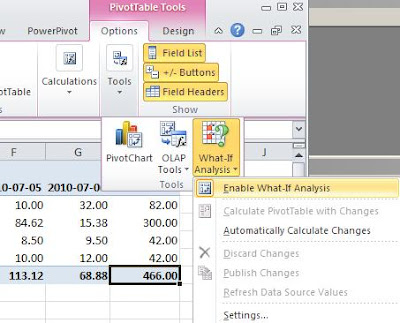 how values are spread, when you enter at a higher level than the cube granularity. For example, you could enter a number for the whole of 2010 and it will spread the amount across all periods based on whether you want an even spread and whether you want the updates to be incremented based on the old numbers.

Excel does not natively support the insertion of new dimension members, which would have been a nice feature for some applications.

Operationally, I don't think it is so important to migrate the writeback data to the main partition, since the writeback partition is typically MOLAP. However, it would not be difficult to move the data over in an SSIS package on a scheduled basis.

Of course, you can restrict read and write access rights based on roles, so, for example, the Australian users can only update the Australian numbers.

It now really is easy to set up an updateable cube and make available to users with Excel 2010.

Improving Excel's Cube Performance

I am often asked to help with Excel's query performance. The cube is fast and efficient, but some Excel queries are slow due to the MDX that Excel is generating.

This is unfortunate, but there a couple of things you can do about it. Let me describe this particular issue. Essentially, you have a dimension with a large number of attributes. In Excel, you have crossjoined many of these attributes on rows, which you feel is reasonable since you have also added a filter so that the query will only return a small number of rows. For example, here is a query of the FoodmartFull database, where I have filtered on just one customer surname (Peacock) and asked for many customer attributes on rows. This query takes 9 seconds for SQL Server 2008 to execute. The reason it takes so long is that the MDX is asking for a crossjoin of all the attributes, at all levels. Note, this issue can be so bad that the results are not returned before timeout.

I have traced the MDX using SQL Profiler. See the MDX in the picture to the right. (I have formatted the MDX. Wouldn't it be a nice thing if SQL EM would format SQL/MDX for us? That's a topic for another blog.) If you execute this MDX, you will receive 3840 rows! That is a huge number, when you consider there is only one customer and Excel is only displaying 1 row. (I asked for a tabular format. But even if I ask for a compact format, I only get 14 rows.) Understandably, this MDX takes 14 seconds to execute.

The reason I chose this particular query is that all of the attributes you see in the Excel report are from the same dimension. Having all these attributes from the same dimension should be very easy for Analysis Services to return quickly, since it can determine, from the dimension, exactly which Customer cells/aggregations it needs.

I can edit the MDX to simply ask for the crossjoin of the leaf members, which will execute in just 1 second. This is much easier for Analysis Services since we are only asking for asingle row rather than 3840. See the second query.

Of course it is not possible to edit Excel's MDX to make the query faster, but we do have other tricks we can employ. Since the problem is that Excel is inefficiently crossjoin-ing all of the attribute hierarchy sets, we can help Excel by creating a "whopper" user hierarchy that includes all (or many) the attributes we want in our report. If we had a Customer hierarchy with these attributes, Excel wouldn't need to ask for any (or so many) crossjoins and the query will be sub second. Of course, I am not suggesting that you create "whopper" hierarchies all over the place, but it is a consideration. Also note, you do not need to create one "whopper" hierarchy, just a couple of multi-attribute hierarchies might do the trick. This is because the cost of adding (or reducing) the number of hierarchies has an exponential effect on query performance. Each attribute you add will crossjoin the new set (it is not a single member set) with all other rows.

Another, much cleaner, option, if possible, is to simply show properties of existing members, rather than ask for a crossjoin. I say, if possible, as this is only possible if the parent attribute is in the report. Naturally, this is much more efficient, as the generated MDX is simply asking for the member properties of existing members (crossjoin not required).

Whenever there is an Excel performance issue, I would encourage you to trace the MDX using Profiler. Even though you can't directly change Excel's MDX, it will help you understand the problem and give you some ideas to work around it.

For a list of Excel PivotTable tips see http://richardlees.blogspot.com/2009/10/excel-2007-olap-pivottable-tips.html

MDX - Group by measure range dynamically

Here is a similar MDX puzzle. The aim is to aggregate members by the range their measure falls into. For example, aggregate cities into ranges (multiples of 1000) of the number of hits.
Of course, you can hand craft the MDX to define each range, but that's not elegant, scalable or flexible. How about some MDX that dynamically creates the ranges?

Here is a solution from my Weblogs database. The query is aggregating the number of hits for all cities with hits in the 0 - 999 range, 1000 - 1999 range etc. See how it uses recursive MDX, very similar to the preceding blog, which aggregates by distinct member_caption. Recursive MDX really is very useful.

Here is what the output looks like. Note; ignore the city name, that is just the last city in the range. The first measure column has the range limit, the second column has the number of cities and the third measure has the total hits for that range.

To view the cube I used, see http://RichardLees.com.au/Sites/Demonstrations

with
member measures.MyRange as
cstr(round(Measures.Hits/1000,0)*1000)+"-"+cstr(round(Measures.Hits/1000+1,0)*1000-1)
set MyCities as
Order(nonempty([Client Host].[Client Geography].[City],Measures.Hits)
,Measures.MyRange,BASC)
member measures.r as rank([Client Host].[Client Geography],MyCities)
member measures.RangeTot as iif((MyCities.item(Measures.r-2),Measures.MyRange)=Measures.MyRange,
Measures.Hits+(Measures.RangeTot,MyCities.item(Measures.r-2)),
Measures.Hits)
member Measures.RangeTotal as
iif((MyCities.item(Measures.r),Measures.MyRange)=Measures.MyRange,
null,Measures.RangeTot)
select {Measures.MyRange,Measures.RangeTotal} on 0,
nonempty(MyCities,Measures.RangeTotal) on 1
from EasternMining

Aggregations Won't Fix Cube Performance

There appears to be a temptation for SQL sales people to demonstrate the aggregation wizard with the impression that it is the tool to solve all performance issues. Unfortunately, it isn't, and I need to dispel that myth.

The aggregation design wizard is not a performance panacea, but it can help. It's like tire pressure in a racing car. The optimal pressure will help performance, but it won't turn a slow car into a fast car.

Let's think about what the aggregation wizard does. The base cube cells only contain values at the intersection of all dimension keys. When a query asks for data at a higher level, AS must derive this data from the base cells by aggregating them. The aggregation wizard determines which of these aggregations to calculate at cube processing time and store on disk. So designing aggregations will impact your cube processing time. The more aggregations you have the longer the cube processing time, and the larger the cube on disk. At query time, if AS does not have the pre-aggregated cell on disk, it will get the lower level cells (these might be aggregations too) and calculate the aggregated cell. This new aggregation will reside in AS memory like any other aggregation or base cell. So there's the rub, even if you don't have any aggregations, AS will create them at query time (or cache warming) and try and keep them in memory for subsequent queries. So, if AS is not memory constrained, aggregations will only help the queries while the cache is cold. In essence, a cube warming query (CREATE CACHE) will have a similar effect as aggregation designs for a non-memory constrained cube.

Cubes that benefit the most from aggregation design are ones that are updated frequently (for example, every minute or so during busy times) and are larger than the memory available to the AS data cache. Note, when a cube partition is processed, all the cells and aggregations in memory are dropped.

Another important note; by default, the aggregation wizard will only create aggregations on key attributes and attributes in natural hierarchies. For example, if you have a Date dimension with date as the key, the aggregation wizard by default, will only build aggregations on "date" and natural hierarchies. If these other attributes are commonly used and you would like the aggregation wizard to consider them, you can ask for it in the Aggregation Usage window (or properties in the cube design). The "Default" usage for a key is "Unrestricted", while the "Default" usage for a non-key property is "None". However, don't see this as a silver bullet, by enabling all properties as "Unrestricted"! That will only result in very thin aggregation design. Also, aggregations on keys, tend to be the most important ones, so the default options suit most cubes.

When using "Distinct Count" measure in a cube you need to be even more careful with aggregations, since each aggregation (and base cell) will include every distinct value of the Distinct Count. This can make aggregations very large and costly to build/query.

For very small non volatile cubes such as the New Zealand census cube http://EasternMining.com.au/sites/Demonstrations/Pages/NZCensus_Excel.aspx there is no benefit from aggregations, which is why that cube has no aggregations.

For really good OLAP cube performance you should ensure that the design is optimal, and use aggregation design (or usage based aggregation design) as a final operational tuning exercise.

MDX is a redundant language

It is often said that SQL is a redundant language, since all but the most simple queries can be written many different ways. Well, I find MDX much more redundant than SQL. There really are thousands of ways to express the same logical query. I like this, since it means that there are lots of opportunities to tune the query by writing it in a different way. Just like SQL. As an MDX writer, I encourage you to strengthen your ability to write queries in different (redundant) ways. This will make you more powerful in query writing and give you more performance opportunities.

Here is a simple example, which involves one of the most common "brick walls" hit by new MDX writers. You want to write a query that would be the logical equivalent of

columnx IN ('Australia','New Zealand'). Here is one way to write this in MDX

with member [Client Host].[Client Geography].ANZ as
sum({[Client Host].[Client Geography].[Region].&[Asia].[AUSTRALIA],
[Client Host].[Client Geography].[Region].&[Asia].[NEW ZEALAND]})
select
{measures.hits,measures.sessions,Measures.[bytes total]} on 0,
tail([Date].[Year Month Day].[Month],12) on 1
from [EasternMining]
where [Client Host].[Client Geography].ANZ

Here is another way to write exactly the same query

select
{measures.hits,measures.sessions,Measures.[bytes total]} on 0,
tail([Date].[Year Month Day].[Month],12) on 1
from
(select {[Client Host].[Client Geography].[Region].&[Asia].[AUSTRALIA],
[Client Host].[Client Geography].[Region].&[Asia].[NEW ZEALAND]} on 0
from [EasternMining])

Of course there are many other ways of expressing this same query. I would not suggest that you should use one technique over the other. It really depends on which one is easier to read, easier to maintain, and runs faster.

For online real-time OLAP and data mining demonstrations goto http://RichardLees.com.au/Sites/Demonstrations

Optimizing Basket Analysis

Basket Analysis is the analysis of sales by basket (or transaction). It can be useful in understanding questions such as

• What is the total value of sales for transactions that include products x (and y, and z...)?
• What is the average transaction value for transactions that include products x (and y, and z...)?
• What proportion of transactions include products x (or y or z)? And what proportion of transactions that include products a (and b, and c...) also include products x (and y, and z...)?
• How did the attach rate of product x change during the sales promotion series? And was there a lasting effect.
• Any analysis that requires mix of products within transactions.

Traditionally basket analysis has been achieved by running SQL queries on very large, highly scalable, databases that dynamically summarize by transaction id. You can imagine that these queries involve huge numbers of transaction and item records and really enjoy massively parallel computers. However, it is now possible to run quite effective basket analysis systems using low cost commodity hardware and Microsoft OLAP cubes. Many people do this by creating a cube with a dimension on the transaction id. If you are considering creating such a solution, I have two major suggestions. This has helped me create basket analysis solutions that consume hundreds of millions of transactions in cubes that support relatively fast ad hoc queries (sub 30 seconds).

1. Rather than creating a dimension on transaction id, create a dimension on basket id. A basket is defined by the unique combination of items. So all the transactions that include items m, n, o and p, would be considered the same basket. Essentially, the basket id can be used as a dimension like the transaction id, but the basket it dimension is a fraction of the size. This makes the solution much more scalable and faster. A basket id dimension table can be created quite simply by creating a bit string with one bit representing each item. For example an 8000 byte string will support 64000 items. There is a little bit of math to create the bit string. but essentially each ItemID can create an exponential of 2 to get its position in the string. ie
   POWER(convert(bigint,2),ItemID). Of course, a bigint can only support 2 to the power of 64, so you will need to do this by a series of 8 byte strings. This would be very very tedious SQL to write, but I found that it is quite easy to write a little SQL to generate the full SQL. Also note, there is no need to keep the full 8000 bytes, it can be a varbinary to the right most byte with an item. See below.


2. The second major suggestion I have, is to create a dimension using an identity column from the basket id table (there is no need to have the varbinary(8000) column in the cube, and write calculated measures for the basket analysis. ie. I would resist using the distinct count physical measures in the cube. You really need a Basket dimension, so that you can identify specific combinations of items.

The result is a relatively small cube, with a relatively large basket id dimension. The cube will have two measure groups, one for transactions with transaction count and sale value, while the item measure group will have item sales value and item count measures. Here is the short SQL query that will generate the full query for the basket ids. It is only a few lines of SQL, but it will generate over 1100 lines of SQL that will form the query for calculating the unique basket id. You will want to run this query incrementally, so just put a where clause at the bottom to ensure it is over the high water mark. I would also encourage you to put the query in an SSIS package with an OLEDB call to a procedure to look up the identity column on the basket table, so that can be stored with the transaction. The rest, including building the cube, should be easy.

A complementary application to this basket analysis cube is a data mining model targeted at the relationships between sales items and useful for predicting sales items.

If you are having performance issues with your basket analysis solutions or want help with your application, don't hesitate to ask me to help. This is the type of BI activity I really enjoy.

For real-time demonstrations of OLAP, data mining and related BI technologies see http://EasternMining.com.au/Sites/Demonstrations

My Calculated Member is slow

Have you written a calculated member that is performing very slowly, while the underlying physical measures are fast? This could be a common cube query performance issue that has a very quick remedy.

Essentially, AS want to know when to treat this as an empty cell. If you don't specify the non_empty_behaviour, AS will need to physically calculate all potential cells to determine which ones are actually emtpy. With non_empty_behaviour specified, AS can avoid many calculations, since many blocks of cells are known to be empty. The non_empty_behaviour attribute is appropriate for both SQL Server 2005 and SQL Server 2008.

To remedy, all you need to do is specify the non_emtpy_behaviour for the calculated member.

Note, there are logic implications with non_empty_behaviour. With the example in the picture (hits per web session) it is logical that I would want to return null when the sessions measure is null. This would not be the case if I were calculating a YTD measure, since the measure might be null on the current day, but the calculation needs to add many other days that might not be null.

For live OLAP and data mining demonstrations with real data see http://RichardLees.com.au/Sites/Demonstrations